Abstract This chapter describes some considerations to use very high pressure instruments in recent times. Smaller particles permit faster separations. To operate columns with small particles, one needs a higher pressure than is possible with classical HPLC instruments. Advantages which can be expected from sub-2-µm particles at pressures up to 1000 bar (15,000 psi) are faster separations with the same resolving power, or a higher resolving power in a realistic time using smaller particle columns and the associated instrumentation.
LevelBasic
If we look back at the history of HPLC, we see that there has been a slow but persistent trend towards smaller and smaller particle size. As a matter of fact, HPLC achieved its breakthrough, when it became possible for the first time to pack particles under 30 µm to prepare efficient HPLC columns [1, 2]. The commercial introduction of 10 µm µPorasil® and µBondapak® columns in 1973 provided a sufficiently attractive separation power to the analytical chemist to make HPLC an effective tool that was competitive to gas chromatography, which was the leading analytical separations tool at that time. Rapidly, packing technologies for still smaller particles were explored [3]. In the first few years, only 10 µm and 5 µm particles were commercially available, and columns packed with these particles were used during the rapid growth of HPLC applications. Then, 3 µm particles became available [4, 5], and in the early 21st century, 3 and 5 µm particles have become the everyday tools of most chromatographers, while still smaller particles sizes became of interest for very rapid analyses.
What is driving this trend towards smaller particle sizes is the desire to achieve the same performance as is possible with larger particles in a shorter analysis time. The time pressures in the analytical lab continue to increase, as the demand for more analyses per unit time and more validation work increases steadily. It can be shown how the reduction in particle size improves the productivity in HPLC [6, 7, 8, 9]. While shorter analysis times are desired [10], one cannot compromise on the separation power of the analysis either, and it is clear that smaller particles are needed in order to maintain the separation power [8, 9]. However, within the realm of classical HPLC, there is a limitation how far one can go with a limited pressure.
Higher pressures are needed to speed up the analysis further while maintaining or even improving the separation power. Higher pressures result in a significant heating of the mobile phase [3]. These thermal effects appeared to pose an upper limit on the pressure that can be used in HPLC, accompanied by a lower limit on the particle size that is still useful [3]. However, investigations by Jorgenson and coworkers demonstrated that there is a way around this problem: the use of smaller diameter columns permits a faster transfer of heat out of the column [11], and much higher pressures can be used than originally anticipated [12, 13, 14]. With the availability of higher pressure, separations with extraordinary separation powers could be accomplished. In the 1997 landmark paper by Jorgenson and coworkers [11], pressures up to 4000 bar were used with small diameter columns packed with sub-2-micron particles. The technique was demonstrated both for isocratic and gradient elution. In the more recent publication [14], porous 1.5 µm ethyl-bridged hybrid particles were used.
Of course, the effort to get to this point was much more challenging than is reflected in these few sentences. Every aspect of chromatography becomes more difficult with increasing pressure. This includes the design of the pumping system and the injection device, and last, but not least, the chromatographic column. But once the feasibility had been demonstrated, the interest rose to put the operation at higher pressure to practical use. This was accomplished with the introduction of the first commercial instrument capable of 1000 bar (15,000 psi) in 2004. The instrumentation and the features of the technique have been described in several articles [15, 16, 17, 18]. Here, the principles will be discussed together with a few application examples.
The reason for the use and the implementation of the principles of very high pressures in LCThe benefits of the use of smaller particles can best be seen by examining plots of plate count versus the time required to accomplish the analysis. In order to do this, we need to fix a few chromatography parameters. We assume that the molecular weight of the analyte is about 250, and that the mobile phase has the viscosity of water at 30°C. This is a reasonable average between solvent compositions that contain acetonitrile and those that contain methanol, and the molecular weight of the analyte is typical for a pharmaceutical analyte. With these suppositions, we can now look at a comparison of the performance of different chromatographic columns in a very straightforward way.
Let us do this first for the simpler case of isocratic separations. A comparison of a series of columns with the same ratio of column length to particle size is shown in Figure 1. We are comparing a 30 cm 10 µm, a 15 cm 5 µm, a 10 cm 3.3 µm, a 7.5 cm 2.5 µm, and a 5 cm 1.7 µm column to each other. The plot displays the plate count achievable at a particular analysis time on the Y-axis, and the retention time of an unretained peak (in minutes) is shown on the X-axis on a logarithmic scale. It can be seen that the maximum plate count that can be realized with all these columns is roughly the same, i.e nearly 13,000 plates, but the time frame is different. For the 10 µm column, the maximum plate count required a column dead time of nearly 30 minutes. For the 5 µm column, the maximum plate count can be achieved in about 7 minutes, which is still fairly large. A reasonable speed is realized with the 10 cm 3.3 µm and the 7.5 cm 2.5 µm columns, with a 3.5 minute or a 1.75 minute column dead time. For a retention factor of 5, the first column would require a 21 minute analysis time, while the second column would complete the same analysis with the same performance in under 11 minutes. A still faster analysis can be accomplished with the 1.7 µm columns. It will take as little as 5.5 minutes.
Column plate count versus the retention time 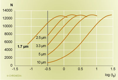 Source: Waters Corporation Figure 1: Plot of column plate count versus the logarithm of the retention time (in minutes) of an unretained peak for columns with an equal ratio of column length to particle size. From the right: 30 cm 10 µm, 15 cm 5 µm, 10 cm 3.3 µm, 7.5 cm 2.5 µm, and 5 cm 1.7 µm. The vertical bar is a pressure limit of 265 bar (4000 psi).
In figure 1, we are also showing the speed limit for these columns, which is imposed by the pressure capability of the HPLC instrument. All curves stop at a column dead time of 20 seconds. This is the point when the pressure limit of the HPLC instrument has been reached. This was set here at 265 bar (or 4000 psi). However, if a higher pressure is available, a still faster analysis can be carried out: the range to the left of the vertical bar is the capability of the increased pressure that the UPLC instrument can offer. Now, the UPLC pressure limit is reached when the column dead time is about 5 seconds. We can compare this to the 10 µm 30 cm column which corresponded to the state of the art at the beginning of HPLC in 1973. The older column achieved the same plate count with a column dead time of about 2.5 minutes. This is a roughly 30-fold improvement in chromatographic speed over a time period of just over 30 years.
This can be demonstrated also and with more clarity than the theoretical graphs above with some simple isocratic chromatograms. In figure 2, we show the reduction in the analysis time for equal resolution going from a 5 µm column to a 1.7 µm column. The scaling was done according to the exact same principles as in figure 1: the column length was reduced in proportion to the particle size, while the flow rate was increased to maintain a constant resolution. The experiment follows the theoretical predictions in figure 1.Isocratic chromatograms with different particle-size columns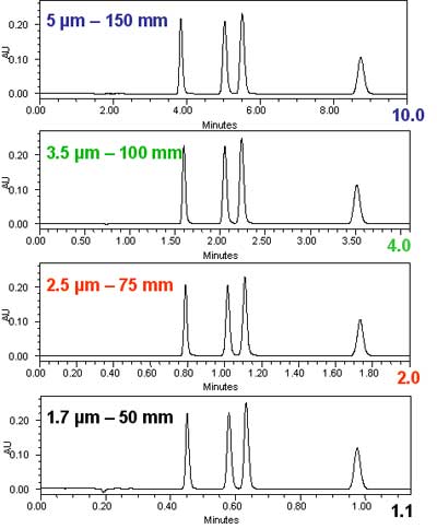 Courtesy of Waters Corporation.
Figure 2: Isocratic chromatograms obtained with different particle-size columns scaled to maintain a constant resolution. The internal diameter of all columns was 2.1 mm. From top to bottom: 1. Column: 5 µm x 150 mm; flow rate: 0.2 mL/min; injection volume: 5 µL. 2. Column: 3.5 µm x 100 mm; flow rate: 0.3 mL/min; injection volume: 3.3 µL. 3. Column: 2.5 µm x 75 mm; flow rate: 0.5 mL/min; injection volume: 2.5 µL. 4. Column: 1.7 µm 50 mm; flow rate: 0.6 mL/min; injection volume: 1.7 µL.
In figure 2, we see without difficulty that the resolution did not change. We measured the resolution between the second and third peak and found it to be absolutely constant at 2.3 for all four chromatograms. However, a few other things changed. Since smaller particles were used in the shorter columns, the injection volume could be reduced with the column volume to maintain the same sensitivity. Note that the injection volume was changed in direct proportion to the particle size, while the signal height remained the same. Most importantly, the analysis time was reduced 9-fold, in exact agreement with the theoretical expectations. The benefits of the reduction in particle size are a higher speed of analysis (= reduced analysis time) and a higher sensitivity (= smaller injection volume).
This set of chromatograms confirms the theoretical expectation discussed above and clearly illustrates one of the reasons for the trend towards shorter analysis time and higher pressure, and one of the two principal reasons for the existence of UPLC.
There is a second factor though, and this is the improvement in the performance of a separation at a fixed analysis time. There is always an optimal particle size and an optimal column length, if we want to maximize the resolution at a single fixed analysis time and a single fixed pressure [19, 20, 21]. But we need to take into account that in reality, one does not vary the particle size by 1/10th of a micrometer or the column length by a millimeter. We need to paint with a broader brush to assess the capabilities of different columns.This is done in Figure 3, where we plot the plate count versus the analysis time for a range of column choices. The red/brown lines and the heavy solid line are columns packed with 1.7 µm particles. Green lines represent 1.0 µm particles, while the blue lines correspond to columns packed with 2.5 µm particles. The column lengths were varied in steps of 5 cm. An increase in plate count is realized for each increase in the column length. For the targeted range of analysis times (between the vertical lines), the 20 cm 1.7 µm column outperforms all other options of particle sizes and column lengths. The maximum performance is around 50,000 plates (the fat red/brown line). Columns packed with the larger 2.5 µm particles can not compete due to the slower mass transfer of the larger particles. The columns with the smaller 1.0 µm particles fail due to the higher pressure requirement that comes along with the use of smaller particles: they do not reach the plate-count maximum any more due to the pressure limitation of 1000 bar. Therefore they can not reach the plate count achieved with the 1.7 µm column in this analysis time. Consequently, only a particle size of around 1.7 µm has the correct properties to deliver a well-functioning column in the desired pressure range. This speaks for an essential feature of UPLC: column design and instrument features, most importantly the particle size and the pressure capability, need to combine well to deliver the right performance features. With other words, the choice of a 1.7 µm particle is a good match for an instrument pressure capability of 1000 bar. On the other hand, if we would not have this pressure capability, 1.7 µm particles would not be the correct choice, and the capability to run fast analyses at high performance would not exist either.
Plot of plate count versus analysis time 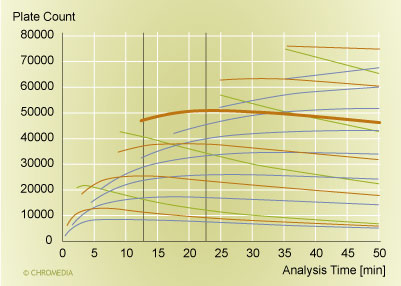 Source: Waters Corporation
Figure 3: Plot of plate count versus analysis time for various column configurations. The pressure limit is 1000 bar, and the molecular weight of the analyte was 150. Mobile phase: water at 30°C. Bold brown line (at 50,000 plates): 20 cm column packed with 1.7 µm particles. Red/brown lines: other columns packed with 1.7 µm particles. Green lines: columns packed with 1.0 µm particles. Blue lines: columns packed with 2.5 µm particles. The column length varies in 5 cm steps.
Essentially the same features as described above for isocratic separations can be observed in gradient separations as well. However, the situation is a bit more complicated. In gradient analysis, the performance of a separation can be measured using the peak capacity: ![]() (1)
(1)
tg is the gradient run time, and is the average peak width. One can either determine the peak width of all peaks in the chromatogram, or (in very complex chromatograms) one can select a few representative peaks to calculate the average peak width.
For a reasonably uniform sample, this can be expanded to read ![]() (2)
(2)
The peak capacity depends on the column plate count and a complex function of the gradient slope G and the gradient run time [22]. If we keep the gradient constant, the peak capacity simply depends on the plate count in exactly the same way as in isocratic chromatography, and all the rules outlined above for isocratic chromatography hold. However, from the practical standpoint it is often better to maintain a constant gradient run time. We will briefly examine here the peak capacity for the case of a complex sample in UPLC. In another paper, we will discuss the intricacies of gradients and peak capacity in gradients [23].
The advantage of a high peak capacity in a reasonable run time for the analysis of complex samples is clear: due to the fact that we obtain a higher chromatographic resolution, interference from neighboring peaks declines. This means that ion suppression, which is a common curse for the LC/MS analysis of such samples, is much lower, and peak identification and quantitation are improved.
In figure 4, below, we show the peak capacity for a 5 cm 1.7 µm column for the analysis of small molecules (MW ~ 150). Plotted is the peak capacity as a function of the flow rate and the gradient run time.
Peak capacity versus flow rate and gradient run time for the analysis of small molecules.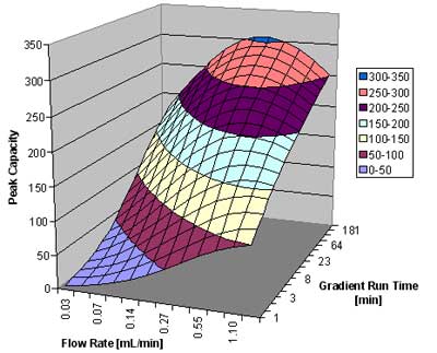 Courtesy of Waters CorporationFigure 4: Plot of peak capacity versus flow rate and gradient run time for the analysis of small molecules.
We can see that the peak capacity increases with increasing run time, but starts to flatten out after about 1 hour. For very rapid gradients, a high flow rate around 1 mL/min gives the best results. For a 15 minute gradient, around 0.5 to 0.6 mL/min is best. For very slow gradients, a flow rate of 0.4 mL/min is recommended. A peak capacity around 200 is readily achievable for a 15 minute gradient, and it reaches a value of just above 300 for the 4-hour gradient for this column.
In figure 5, we show the peak capacity for a peptide sample with an assumed average molecular weight of 2000, over a gradient span of 50% organic in the mobile phase. The column is a 5 cm 1.7 µm column, as above. Of course, for a separation of compounds with a large molecular weight, a rapid gradient does not promise to result in high resolution. On the other hand, a gradient over 4 hours at a flow rate of around 0.1 mL/min gives superb results: a peak capacity close to 600 can be achieved under these circumstances. A column packed with 3.5 µm particles would only result in about half the resolution; an optimal peak capacity of only around 350 is predicted.
Peak capacity as a function of flow rate and gradient run time for a peptide sample. 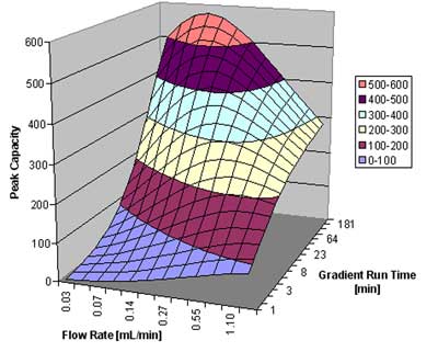 Courtesy of Waters Corporation
Figure 5: Peak capacity as a function of flow rate and gradient run time for a peptide sample.
In figure 2 above, we have demonstrated the advantage of the use of smaller particles with a very simple analysis of 4 standards. The same advantages found with the standards have also been established with realistic samples. A good example of this is shown in figure 6.Example of the transformation of an isocratic analysis from an HPLC column (top) to a UPLC column (bottom). Click to enlarge)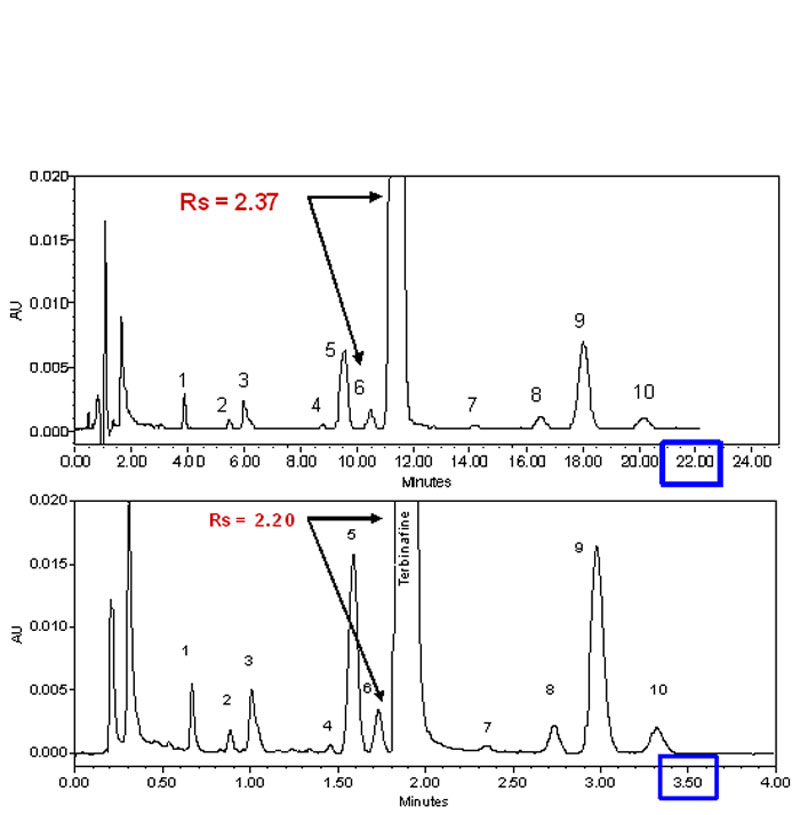 Courtesy of Waters Corporation
Figure 6: Example of the transformation of an isocratic analysis from an HPLC column to a UPLC column. HPLC (top) 2.1 x 150 mm 5 µm XBridgeTM C18, flow rate 0.3 mL/min. UPLC (bottom): 2.1 x 50 1.7 µm ACQUITY UPLC® BEH C18, flow rate 0.6 mL/min. Instrument: ACQUITY UPLC® with TUV optical detector. Chromatographic conditions: mobile phase A: 20 mM ammonium bicarbonate pH 10.0, mobile phase B: acetonitrile; isocratic: 73% B.
The separation scaled perfectly from the 15 cm 5 µm column to the 5 cm 1.7 µm column, with essentially the same resolution between the parent peak Terbinafine and the closely eluting impurity in front of the main peak. The analysis time was reduced from 22 minutes for the HPLC column to about 3.5 minutes on the UPLC column, a 6-fold increase in the speed of the analysis, with no drawbacks. Many similar application examples have been generated, confirming the theoretical predictions of the advantages of smaller particles in short columns.
An application example with a gradient separation is shown in figure 7. We are comparing here the same separation obtained on a column with a 5 µm particle to one obtained under the same conditions with a 1.7 µm ACQUITY UPLC® BEH C18 column. One can see without difficulty the improvement in resolution. The peak capacity estimate yielded a value of 140 for the classical column, and 360 for the UPLC column.
Separation of a protein hydrolysate on two columns with different particle sizes. (Click to enlarge)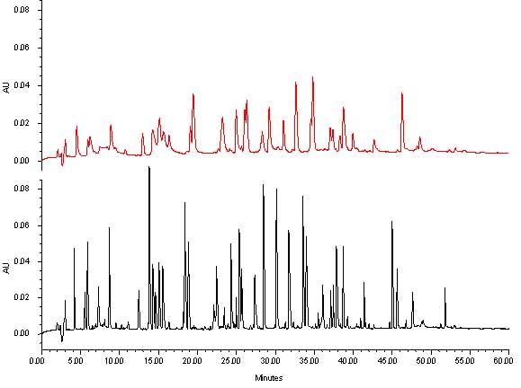 Courtesy of Waters Corporation
Figure 7: Separation of a protein hydrolysate on two columns with different particle sizes. Top, experimental 5 µm column, 2.1 x 100 mm. Bottom ACQUITY UPLC® BEH C18, 2.1 x 100 mm, 1.7 µm. Mobile phase A: 0.02% TFA in H2O. Mobile phase B: 0.016% TFA in acetonitrile. Flow rate: 0.1 mL/min. Gradient: 5% to 45% B in 60 minutes. Sample: MassPREPTM Enolase Digestion Standard. Temperature: 38°C. Instrument: Waters ACQUITY UPLC® 250 nL Capcell TUV detector.
This example demonstrates another feature of the application of small particles. Note that in this case, a very simple comparison was done, using just two different particle sizes with the same application and the same column length. To match the performance of the small-particle column, one would have needed to increase the column length 3 times and to run a 3-times longer gradient. The first requirement is possible; the second requirement results in a prohibitively long analysis time. A standard gradient analysis of 3 hours is not a conditions that most practitioners would select. On the other hand, a 1-hour analysis time for a peptide sample is nothing unusual, and the advantage that one gets from the smaller particles are welcome.
- J. J. Kirkland, J. Chromatogr. Sci. 10 (1972), 593
- R. E. Majors, Anal. Chem. 44 (1972), 1722-1726
- I. Halász, R. Endele, J. Asshauer, J. Chromatogr. 112 (1975), 37-604.
- J. L. DiCesare, M. W. Dong, L. S. Ettre, Chromatographia 8 (1981), 257-286
- M. W. Dong, J.R. Gant, LC/GC 2 (1984), 294- 302
- U. D. Neue, J. L. Carmody, Y.-F. Cheng, Z. Lu, C. H. Phoebe, and T. E. Wheat, “Design of Rapid Gradient Methods for the Analysis of Combinatorial Chemistry Libraries and the Preparation of Pure Compounds”, in Advances in Chromatography, Edited by E. Grushka and P. Brown, Vol. 41, 93-136, Marcel Dekker, New York, Basel, 2001
- Y.-F. Cheng, Z. Lu, and U. D. Neue, “Ultra-Fast LC and LC/MS/MS Analysis”, Rapid Commun. Mass Spectrom. 15 (2001), 141-151
- U. D. Neue, B. A. Alden, P. C. Iraneta, A. Méndez, E. S. Grumbach, K. Tran, D. M. Diehl, “HPLC Columns for Pharmaceutical Analysis”, in Handbook of Pharmaceutical Analysis by HPLC, M. Dong, S. Ahuja, Editors, pp. 77-122, Academic Press, Elsevier, Amsterdam, 2005
- U. D. Neue, Y.-F. Cheng, Z. Lu, “Fast Gradient Separations”, in “HPLC Made to Measure: A Practical Handbook for Optimization”, Stavros Kromidas, Ed., pp. 47-58, Wiley-VCH, Weinheim, 2006
- P. R. Tiller, L. A. Romanyshyn, U. D. Neue, “Fast LC/MS in the analysis of small molecules”, Analytical and Bioanalytical Chemistry 377 (2003), 788-802
- J. E. MacNair, K. C. Lewis, J. W. Jorgenson, Anal. Chem. 69 (1997), 983–989
- J. E. MacNair, K. D. Patel, J. W. Jorgenson, Anal. Chem. 71 (1999) 700–708
- K. D. Patel, A. D. Jerkovich, J. C. Link, J. W. Jorgenson, Anal. Chem. 78 (2004), 1697-1706
- J. S. Mellors, J. W. Jorgenson, Anal. Chem. 2004, 76, 5441–5450
- J. R. Mazzeo, U. D. Neue, M. Kele, R. Plumb, “Advancing LC performance with smaller particles and higher pressures”, Anal. Chem. 77(23) (2005), 460A-467A
- U. D. Neue, E. S. Grumbach, M. Kele, J. R. Mazzeo, “Ultra-Performance Liquid Chromatography”, in “HPLC Made to Measure: A Practical Handbook for Optimization”, Stavros Kromidas, Ed., pp. 470-477, Wiley-VCH, Weinheim, 2006
- U. D. Neue, „Ultra-Performance Liquid Chromatography“, Encyclopedia of Separation Science, in print
- M. E. Swartz, J. Chromatogr. Rel. Technol. 28 (2005), 1253-1263
- M. Martin, C. Eon, G. Guiochon, J. Chromatogr. 99 (1974), 357-376
- M. Martin, C. Eon, G. Guiochon, J. Chromatogr. 108 (1975), 229-241
- M. Martin, C. Eon, G. Guiochon, J. Chromatogr. 110 (1975), 213-232 22. U. D. Neue, J. Chromatogr. A 1079 (2005), 153-161
- U. D. Neue, Gradients in RPLC, Chromedia
- U. D. Neue, Hybrid Stationary Phases for RPLC and the Use of these Packings in Method Development, Chromedia
- M. Martin, G. Guiochon, J. Chromatogr. A 1090 (2005), 16-38
